|
|
|
|
|
In this section (as well as below), we shall present the basic astrophysical
results obtained in Experiment cold. Some of the results have already been
published in short papers (Pis'ma v Astron. Zh. [Sov. Astron. Lett.],
abstracts of papers read at international conferences, etc.), some
are published here for the first time, and for some problems, the observations
have not yet been completely reduced so that we can only give preliminary
conclusions. First of all, we shall discuss the results of the deep sky
survey.
7.1. General Characteristics of the Region Surveyed
As we said above, the main subject of our research was the strip of
sky within ![]() 10' of the line on the celestial sphere with d
= dSS433= 4o54'. This
strip is depicted in Galactic coordinates in Fig. 7.1. The strip studied
passes through the Milky Way twice: through the region W50 (and SS433)
and near the Rosette Nebula (W16), where the background emission of the
Milky Way is much fainter and was not detected at centimeter wavelengths.
A significant portion of the strip is located at high galactic latitudes,
reaching b11= 68o, and it passes through the coldest
regions of the northern sky.
10' of the line on the celestial sphere with d
= dSS433= 4o54'. This
strip is depicted in Galactic coordinates in Fig. 7.1. The strip studied
passes through the Milky Way twice: through the region W50 (and SS433)
and near the Rosette Nebula (W16), where the background emission of the
Milky Way is much fainter and was not detected at centimeter wavelengths.
A significant portion of the strip is located at high galactic latitudes,
reaching b11= 68o, and it passes through the coldest
regions of the northern sky.
It is difficult to reproduce a sample of a single 24-h long scan here
because of the large dynamic range of the observed phenomena. Atmospheric
emission frequently causes powerful background phenomena, although in sufficiently
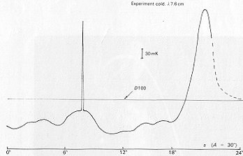
good weather, the Galactic background dominates. A 24-h-long scan of this
strip of sky during observations at an azimuth of 30o (Experiment
Cold-2) in 1981 is shown as an example in Fig. 7.2. The horizontal line
is the sensitivity limit of the Bonn 100-m paraboloid in Galactic surveys.
In addition to the background radio emission, some features are visible
on individual scans – sources and interference. Comparing two diurnal scans
allows one to estimate that about 400 features repeat from day to day.
We call the repeatable features which are visible on individual scans "strong"
sources. Those features (sources) which are visible on an individual 24-h-long
scan are shown in Fig. 6.3 (upper portion). In the lower portion of the
figure, individual sections of the same strip of sky are shown, but after
prolonged averaging: the section between a =
13h
and 14h,
and a small portion of the section between a
= 13h
and 14h
are shown under high magnification.
7.2. "Strong" Radio Sources
Features with a peak flux density of about 10 – 15 mJy (at the 2s- level) are visible on individual records. Table VII.I compares this with the major complete all-sky surveys.
As is evident from this table, all of the sources with a normal spectral
index ( P ![]() ma ,
a = – 0.7 ) in all the major
catalogues should be detected, even in a single 24-h-long scan; this is
even more true for sources with excess radio emission at high frequencies.
The majority of the "strong" sources detected in the Cold survey are new.
We note that the diurnal information flow (number of radio sources) in
Experiment Cold was almost equal to the total number of radio sources with
P < 0.2 Jy that have ever been observed using all of the radio telescopes
ma ,
a = – 0.7 ) in all the major
catalogues should be detected, even in a single 24-h-long scan; this is
even more true for sources with excess radio emission at high frequencies.
The majority of the "strong" sources detected in the Cold survey are new.
We note that the diurnal information flow (number of radio sources) in
Experiment Cold was almost equal to the total number of radio sources with
P < 0.2 Jy that have ever been observed using all of the radio telescopes
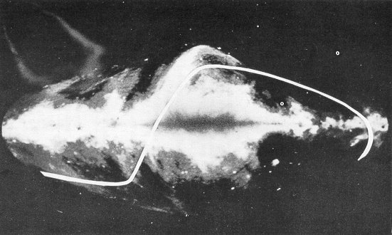
Figure 7.1 The position of the deep-survey band in Galactic
coordinates. The band studied is superposed on a radio image of the Galaxy
obtained through the joint efforts of radio observatories at Effelsberg,
Jodrell Bank, and Parkes.
taken together. At the beginning of 1982, this number was 495 (Pauliny-Toth, 1982).
The data on the log N – log P curve will be given below; the average
number of "strong" sources with P > 7.5 mJy in a 1-h zone of right ascension
is ~ 15 ![]() 4. These sources are distributed uniformly over the 1-h intervals, within
the errors.
4. These sources are distributed uniformly over the 1-h intervals, within
the errors.
| Name
Cambridge, 3C
|
|
|
|
|
|
|
The distribution of sources with flux densities P > 7.5 mJy, obtained from an examination of individual 24-hour-long scans over the area 0h < a < 24h is shown in Table VII.III. This table will be used in the next section to construct the log N – log P curve. A complete catalog of all the observed sources will be published separately.
We shall now present preliminary results on the statistics of radio sources with flux densities P > 0.86mJy. Examples of the individual
|
|
|
|
|
|
|
|
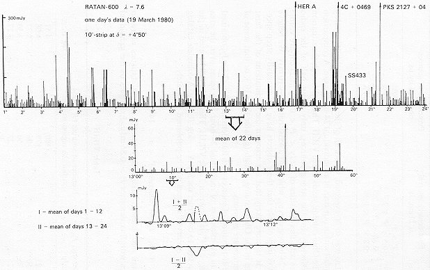
Figure 7.3 One day's data on discrete radio sources obtained at 7.6cm (upper curve). On averaging scans, fainter sources (see the section from 13h<a < 24h below) become visible with the increase in sensitivity. Below this, a section several minutes long is shown at a higher scale: the average and half-difference of two groups of scans showing that almost all of the features are sources.
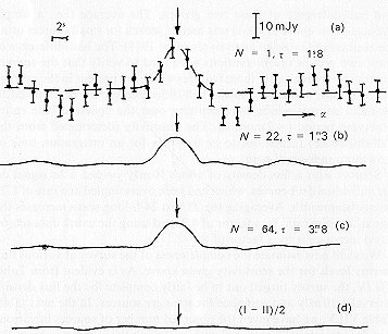
Figure 7.4 An example of a drift scan through a source
with a flux density of 10mJy. (a) A single scan with an integration time
of 1.8 s. (b) An average of 22 scans, with an effective integration time
of 40s. (c) Average of 64 scans using observations at the meridian and
azimuth 30o; the effective integration time is 1.9 min. (d)
The difference between the data from two 11-day observing cycles (cycle
I and cycle II). The absence of a signal in the difference curve is taken
as proof that the radio source is real.
and averaged scans of the radio emission of the sky at 7.6 cm are shown in Figs. 7.3 and 6.2. Sources not visible on an individual scan were detected in the averaged set of data. We remind the reader that about 70 24-h-long scans of the strip of sky being studied were obtained in all; in principle, this allows flux densities of about 1 mJy to be recorded. Not all of the scans proved to be of high quality. Therefore, the first step consisted of removing the bad scans. Thus, we chose 22 scans of fairly high quality out of all the scans of the section 13h <a < 24h made at the meridian in 1980 (Experiment Cold-1). An example of a small section of such a scan is shown in Fig. 7.4. The data reduction program allowed the background to be subtracted (via a moving average), leaving only the small-scale (for example, those smaller than 10') features. After a preliminary cleaning of the individual scans – removal of ordinary strong interference we divided all of the scans of the section 13h<a < 24h into two groups of 11 days each, averaged them and constructed the average and half-difference of these two groups. The average (i.e., a simple average of the entire 22 days) was used to search for small sources using the method of Gaussian analysis (Ivanov, 1979). The half-difference of these two groups of observations were used to verify that the sources observed were real: only those features which are present in the average of the groups and absent in the half-difference should be assumed to be radio sources which were emitting over the course of the entire observing period (~ 2 months). The sensitivity (determined from the half-difference) turned out to be 0.64mJy for an integration time of 3.6 s in an individual scan.
Sources with a flux density of about 10mJy yielded a 3s signal on the individual drift curves, which had been oversampled at a rate of 1.25 points/beamwidth. Averaging the 22 best 24-h-long scans increases the signal-to-noise ratio by a factor of 4.7, and using the entire data set (64 days) increases it by a factor of 8.
We shall now estimate the completeness of the survey at various flux density levels for the sensitivity given above. As is evident from Table VII. IV, the survey turned out to be fairly complete for the flux density interval 1-10mJy and complete for stronger sources. In the next table, Table VII.V, we have given the observed number of sources in various flux density intervals with and without taking the completeness of the survey into account. On the basis of this table, we determine the number of sources with flux density greater than a given value (Table VII.VI).
The "number of sources – flux density" curve (combining the data on "strong" and "weak" sources) is shown in Fig. 7.5, together with the data from the extremely deep survey carried out by Pauliny-Toth et al., at Bonn. It is evident that the log N – log P curve is in extremely good agreement with the Bonn data over the range of flux densities in common; however, its behavior changes drastically for extremely faint sources, approaching "saturation" at a level of 2 x 10⁵ sr-1
Two conclusions follow from Fig. 7.5:
(1) The centimeter-wavelength "number of sources – flux density"
|
|
|
|
|
|
|
|
|
|
|
|
|
|
|
|
|
|
|
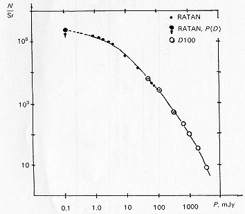
Figure 7.5 The behavior of the log N – log P curve over the entire range of flux densities studied at 7.6 cm: The results of the direct source counts in Experiment Cold are indicated by dots, and the results of the counts from observations at Bonn by circles. It is evident that the data are in good agreement within the region in common.
(2) Our "number of sources – flux density" curve is in good agreement with the results of the Bonn survey (Pauliny-Toth et al., 1978) at a nearby wavelength for P > 15 mJy, as well as the results of the deep 408 MHz surveys at Cambridge. Pooley and Ryle (1968) give data on the behavior of the statistics of sources at 408 MHz with flux densities greater than 15mJy. Such sources will have a flux density of about 3mJy at 7.6cm if they have a normal spectrum. Therefore, the agreement between our "number of sources – flux density" curve and Pooley and Ryle's results indicates that this curve is independent of frequency, at least in the flux density range 3 < P < 100mJy.
7.4. A New Population of Radio Sources?
We shall now discuss the problem of the search for a "new population" of radio sources. As we noted above, such a population was observed by Wall et al., in the flux density range 1 – 15 mJy, but these suspicions turned out to be erroneous. The situation is more complex for very faint objects (fainter than 1 mJy at 7.6cm). Two reports of a sharp break in
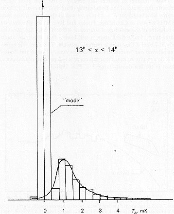
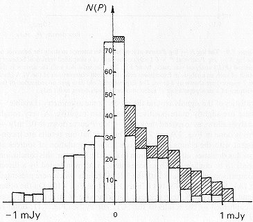
Figure 7.8 The statistics of the readings within the "mode"
(see Fig. 7.7): 450 readings with amplitudes smaller than 1 mJy show some
asymmetry in their distribution, with an excess of positive readings (83
readings within a solid angle of 3.4 x 10⁻⁴sr). This information
was used to obtain the point between 0.1 and 0.2mJy in Fig. 7.9 [P(D) analysis].
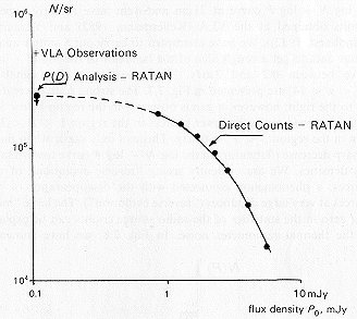
Figure 7.9 The log N – log P curve at low fluxes. An attempt to study the behavior of the log N – log P curve at P ~ 0.1 mJy on the basis of a simplified version of Scheuer's method [P(D) analysis] was made, using Fig. 7.8. The solid dot with the arrrow is the result of such an analysis in Experiment cold; the recent observations at the VLA (data on 7 sources) are shown by a cross. The Experiment Cold data give no indication of the existence of a new population of radio sources at levels down to 0.1 mJy.
statistics of the signals around the mode. Some asymmetry is visible
– there are slightly more positive signals than negative. A very rough
analysis allows us to extend the log N – log P curve down
to 0.2 m Jy – this is done in Figs. 7.9 and 7.5. We believe that our results
are inconsistent with the claims that there is a "new" population of sources
at low flux densities, all the way down to 0.2 m Jy; however, this conclusion
needs to be confirmed. This inconsistency is demonstrated by a direct comparison
of our results with the NRAO results which were presented at IAU Symposium
No. 104 (Crete, 1982) (see Fig. 7.10). On the other hand, the extremely
steep decrease in the number of faint radio sources is confirmed by the
results of the 5C12 survey (see Fig. 7.11, Bonn et al., 1982).
And so, our principal unexpected result from 1980 – a dramatic decrease
in the number of faint radio sources (down to ~ 1 mJy) – is confirmed by
direct counts in 1982 at the NRAO, Westerbork, and Cambridge. The situation
with respect to a "new population" of radio
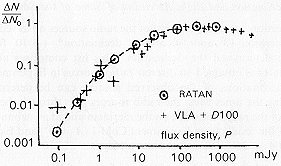
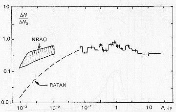
Figure 7.70 A comparison of new (1982) VLA data (6cm)
with 1980 RATAN-600 observations (7.6 cm). Here, DN/N0
is the ratio of the observed differential source density to that expected
for a static Euclidean Universe. The agreement between the RATAN-600 and
VL,4 fata is satisfactory for flux densities greater than 1 mJy. The data
differ by a factor of 3 – 5 at 100 mJy; the
point obtained at the VLA can be interpreted as evidence for the appearance
of a new population of radio sources.
sources (P << 1 mJy) remains unclear at present. Studying the
luminosity function of nearby objects which emit at radio wavelengths shows
that below 100 mJy, the sky should be filled with nearby, faint sources
– faint radio galaxies, as well as normal galaxies. We shall return to
this problem later.
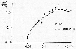
Figure 7.11 Data from the SC12 survey (1982) al 73.5 cm.
Down to the limiting flux of ~10mJy, the curve repeats the 7.6cm observations
(1980), but is shifted in the flux-density scale). The steep slope of the
curve at faint fluxes supports the idea that we have reached a region where
"reverse evolution" of radio sources occurs.
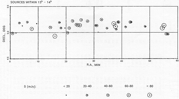
7.5. Declination and Right Ascension of Some of the Sources
In this section, we shall give a list of the radio sources observed between right ascension 13h and 14h around declination* + 5o10' for which we have determined the declination. This list comprises about 5% of the material obtained on discrete radio sources in Experiment Cold.
The declinations of the observed sources can be determined by comparing the times when the radio sources pass through the antenna pattern of the radio telescope on the meridian and at an azimuth 3, i.e., by using the results from Experiment Cold-1 (A= 0o) and Experiment Cold-2 (A = 30o). We call sources all signals which:
(1) exceed the noise dispersion by a factor of 10;
(2) are present in two independent averages of two
groups of observations on the meridian and at an azimuth of 30o
with similar flux densities; and
(3) have declinations (determined from the time
at which they pass through the meridian and azimuth A = 30o
) which agree with the observed times at which the radio sources pass through
the antenna pattern. This time is a known function of how far the source
is in declination from the electrical axis of the antenna pattern (see
Fig. 3.8). The error in determining the times at which the radio sources
pass through the beam of the radio telescope on a single scan is 0'.8 for
sources with a flux density of 5 may, and less than 0';1 for flux densities
of 50mJy. Therefore, the random error in determining the times from an
average of 38 24-h long scans is less than 2", and 2."4 from an average
of 26 scans at A = 30o . The position of the beam of
the radio telescope on the meridian and at azimuth 30' was determined using
the sources 4C05.43 and 4C05.53. We adopted the following coordinates for
these sources:
|
|
|
|
|
No. |
a1950.0 |
d1950.0
|
P
mJy 4 |
f
arcmin 5 |
Notes 6 |
| 1
|
13h 00m 49s:96
13 02 01.98 13 03 14.75 13 04 18.66 13 06 05.97 13 07 42.90 13 09 27.43 13 14 21.91 13 15 58.41 13 17 34.98 13 18 07.72 13 19 33.23 13 20 29.74 13 21 06.04 13 22 17.64 13 23 39.00 13 24 11.40 13 24 56.77 13 28 23.09 13 27 39.37 13 30 35.42 13 30 56.49 13 31 31.23 13 32 40.94 13 34 39.36 13 37 07.95 13 37 42.28 13 37 56.67 13 38 34.47 13 38 47.43 13 41 20.84 13 43 02.67 13 43 16.89 13 48 20.69 13 54 30.12 13 55 07.58 13 55 56.31 13 56 33.94 |
4o 59'07."5
4 59 27.1 5 11 09.1 5 07 43.7 5 12 05.0 5 04 23.5 5 10 17.6 5 06 02.0 4 55 45.1 5 11 37.0 5 05 16.9 5 05 03.3 5 59 41.5 5 05 13.3 5 13 23.7 5 09 05.7 5 08 37.4 5 08 29.5 5 14 32.6 5 13 10.0 5 08 08.4 5 08 01.0 5 00 16.1 5 14 54.3 5 04 56.0 5 10 16.3 5 06 54.6 5 03 42.2 5 12 5 12 5 06 23.7 5 12 5 12 5 06 55.1 5 05 01.8 5 08 09.4 4 58 17.6 4 58 02.8 |
58
|
1
0.5 1 0.5 1 0.5 0.5 0.5 2 0.5 1 0.5 2.2 0.5 1 2.9 3.5 0.5 1 2.7 0.5 0.9 0.5 1 2.3 1 0.5 1 1 1 0.5 2 2 0.5 4.4 0.5 1 1 |
Double Blend?
Multiple? |
| NN | Right ascension
(1950.0) h m s |
|
Anglar size
(') |
| 1
|
13
13 13 13 13 13 13 13 13 13 13 13 13 13 13 13 13 13 13 13 13 13 13 13 13 13 13 13 13 13 13 13 13 13 13 13 13 13 13 13 13 13 13 13 13 13 13 13 13 13 13 13 13 13 13 13 13 13 13 13 13 13 13 13 13 13 13 13 13 13 13 13 13 13 13 13 13 13 13 13 13 13 13 13 |
0
0 1 2 3 4 4 4 5 5 24 25 25 25 26 27 28 28 29 29 30 30 31 31 32 32 33 34 36 36 37 37 37 38 38 39 41 43 43 44 45 45 46 48 48 49 49 49 50 51 52 53 53 54 55 55 56 56 |
50.6
56.1 47.7 4.9 18.4 1.7 21.8 49.0 24.6 48.3 8.1 14.4 47.3 1.4 40.2 54.5 32.1 1.6 15.4 32.8 26.6 54.5 17.3 25.2 5.3 1.7 18.5 39.1 12.1 37.8 34.5 1 1.2 19.3 43.2 41.4 16.7 42.2 4.5 26.0 45.7 41.0 47.2 11.6 59.3 9.7 51.8 39.1 59.7 16.1 35.2 7.5 44.0 56.9 39.9 24.6 51.0 13.2 46.6 57.6 38.8 51.2 33.9 24.5 6.7 21.4 58.7 18.2 36.0 47.7 7.0 25.2 3.7 13.1 47.5 37.6 46.9 36.0 0.1 49.8 33.2 11.5 27.4 13.3 56.1 |
0.008
0.011 0.008 0.009 0.008 0.012 0.008 0.005 0.008 0.005 0.011 0.008 0.030 0.007 0.010 0.017 0.010 0.002 0.012 0.011 0.008 0.007 0.005 0.017 0.006 0.015 0.005 0.011 0.009 0.039 0.009 0.017 0.026 0.006 0.016 0.010 0.011 0.040 0.016 0.006 0.005 0.008 0.005 0.006 0.007 0.010 0.016 0.015 0.005 0.008 0.004 0.012 0.019 0.007 0.009 0.006 0.034 0.055 0.009 0.011 0.017 0.014 0.018 0.006 0.006 0.020 0.019 0.007 0.005 0.004 0.013 0.023 0.042 0.004 0.023 0.006 0.009 0.004 0.005 0.022 0.078 0.006 0.004 0.008 |
2.3
< 0.4 1.4 < 0.5 2.0 2.9 < 0.3 < 1.7 < 3.1 < 0.5 < 2.4 2.7 < 1.1 < 1.4 1.2 1.5 < 0.5 < 2.6 < 1.6 < 1.1 < 2.6 < 3.0 < 1.0 < 1.9 < 1.9 < 4.6 < 1.4 1.2 < 1.3 1.4 < 2.9 1.3 2.1 < 1.5 3.9 < 1.7 < 0.5 1.1 < 5.8 < 1.2 < 0.5 < 2.3 < 0.8 < 1.8 < 1.8 < 1.5 < 1.6 < 0.8 < 4.5 < 0.5 < 4.0 < 2.3 < 0.5 < 3.5 < 1.3 < 1.4 1.8 1.0 < 3.1 < 0.9 < 2.2 < 2.5 < 0.7 < 1.4 < 1.3 < 0.6 < 3.9 < 1.9 < 1.3 < 1.2 < 0.5 < 2.7 4.7 < 8.5 < 2.3 < 0.9 < 0.5 < 2.3 < 2.1 < 4.7 < 0.9 < 1.5 < 2.0 < 1.5 |
{a) source numberThe catalog given in Table VII.VII is not complete, but it contains those sources which were positively detected on the averaged curves and for which the declinations were determined. The overwhelming majority of the sources is new; optical identifications are needed to determine their nature. Their distribution over the section between 13h and 14h is shown schematically in Fig. 7.12. The diameter of the circle is proportional to flux density. In addition, the right ascension and peak flux densities of all sources stronger than few mJy are listed in Table VII.VIII for 13h < a < 14h .
(b) right ascension
(c) declination
(d) flux density P in millijanskys
(e) estimated size, f, in arcminutes.