|
|
|
|
|
As is clear from what was said above, various types of interference
(which differ a great deal in their characteristics) appear when observing
on different spatial scales. Therefore, the problem of approaching the
sensitivity of an "ideal" radiometer must be solved differently depending
on the scale we are interested in. We shall discuss three cases here: scales
comparable to the beamwidth of the radio telescope, scales of order 10
arcmin (10 beamwidths), and large scales (a few degrees and larger).
6.1. Point Sources, i.e., Scales Comparable to the Beam of the Radio Telescope
Research on these scales involves point sources, their distribution on the sky as well as in distance, and as well as their identification and physical properties. The main things which interfere with the identification of sources are noise spikes, confusion noise, and, to some extent, anomalous low-frequency noise.
6.1.1. Noise Spikes. Noise spikes can be divided into two categories:
short noise spikes (d-functions), and noise
spikes comparable in duration to the time required for the sky to pass
through one beamwidth. In order to be able to identify and remove the short
noise spikes, some oversampling was retained in the sampling rate as it
was increased. Because of this, an isolated outlier (for example,
a malfunction in the data collection system, etc.) cannot be a radio source,
since a source with TA = 5s
should occur in three adjacent pieces of data (at 7.6 cm) when the interval
between readings is decreased to 1s.8. Isolated outliers were
removed both automatically and by the observer. While examining the compressed
data set on a computer screen, the observer gives the numbers of the neighboring
readings, and the computer interpolates and replaces the outliers by the
average of the neighboring readings. At this point, one should remember
that a d-function has a white-noise spectrum
wherever it is located in the set of data. Therefore, spectral cleaning
methods are totally inapplicable to noise spikes (as well as the problem
of removing discrete sources from the data set). The energy of a noise
spike is distributed over all frequencies and no spectral filter is able
to remove the interference. This is the hidden danger in the blind use
of Fourier methods by the inexperienced observer when reducing data (without
preparing the data beforehand). Therefore, special methods of dealing with
localized interference must be used in addition to Fourier methods for
interference distributed throughout the data set. Interference of longer
duration (which could be mistaken for a source) was removed by correlating
all the signals above the Scan level on two independent
scans of the same section of the sky. If a signal was present on only one
scan, it was discarded and replaced by an interpolated value. For the section
of sky 13h
< a <
14h,
this procedure was carried out by comparing all of the individual scans
with one another and removing all of the sufficiently strong outliers
using the coincidence principle. One type of interference – faulty automobile
ignitions – instilled great fear and, as was noted above, we expected to
use the 31-cm observations to clean the 7.6-cm records. However, it turned
out that this interference was generally not observed at 7.6 cm, since
this type of interference has a very steep spectrum and the antenna was
protected by antinoise screens.
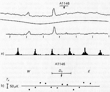
6.1.2. Confusion noise and the number of sources – faux density Relationship It seemed as if confusion noise would be the main limitation in our observations of both point sources and the background radiation. To illustrate this effect, a scan (obtained at 6cm on the Bonn 100-meter radio telescope in a two-beam observing mode (Wall et al., 1982)), which looks like a broad noise tracing with a root-mean-square fluctuation of 2 – 3 mJy, is shown in Fig. 6.1(a). A simple extrapolation (using the formulae given in Section 4.3) to the observations with the north sector of the RATAN indicates that this effect should amount to approximately 2mJy. However, the confusion noise unexpectedly turned out to be significantly lower, because of the following: first, the excess resolution of the sector in the Experiment Cold observing mode, and second, the fact that the eOect is significantly different at flux levels of 1 mJy, and a simple extrapolation according to the recommended formulae (which are based on rougher surveys) leads to an overestimate of the confusion noise.
Radio astronomers have become accustomed to the idea that faint sources are much more numerous than strong sources; the numerical ratio is determined by the log N – log P curve. However, a direct count of the faint sources in Experiment Cold indicated that we are on a rather flat section of the cumulative log N – log P curve (Fig. 6.5),
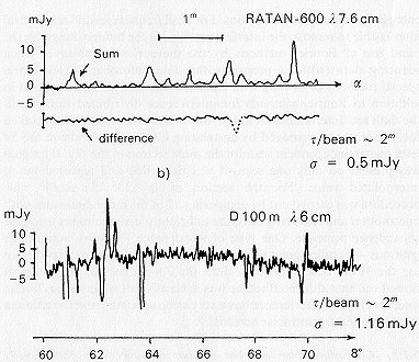
so that the situation is reversed. Thus, in a scan of the section of sky with right ascension 13h < a < 14h within the band surveyed (10' wide in declination at d = 4o 54') averaged over 2 months, the maximum number of peaks due to sources is at amplitudes of 2 – 3 mJy, and there are significantly fewer peaks at a level of 1 m Jy! Direct measurements of the log N – log P curve at fluxes of about 1 mJy have only recently begun. The first such counts were obtained in Experiment Cold-1 in the spring of 1980 (Berlin, et al., 1980). They yielded a significant difterence (up to a factor of 10) toward a smaller number of sources than in the extrapolated estimates. VLA observations (Kellerman, 1982) with a sensitivity several times higher, but based on a smaller statistical sample (a small region with 13 sources), confirmed our results in the 1 mJy flux range (see Fig. 7.10). If one assumes that most sources have a nearly normal spectrum (there is no direct information on the spectra of such faint sources), data at longer wavelengths also confirm our conclusion that the number of sources with fluxes of ~1 may at a wavelength of 7.6cm is small. This explains the pronounced difference in the appearance of the drift curves in the "Cold" cycle compared with Fig. 6.1(a), for example. The average and half-difference of two independent averages over 11 days of observations are shown in Fig. 6.1(6); it follows from these two averages that essentially all of the peaks visible in the scan are sources. Moreover, regions free of sources exist, since only 20% of the space on the scans is occupied by the radio images of sources at the RATAN-600's beamwidth (1 are-minute) and a sensitivity of approximately 1 – 3 mJy; the fluctuations determined by the system noise temperature Tn dominate (the size of the fluctuations can be calculated from Eq. (4.1)) between the sources. This is also demonstrated in Fig. 6.2, where the upper curve is an average of 38 days' observations of the section of sky between right ascensions 13h 52m and 13h 54m, and the lower is the same section after removal of low-frequency noise. Seven sources, as well as regions free from sources with root-mean-square fluctuations of approximately 0.5mJy (which corresponds to the radiometer noise) are visible in this section. Thus, the sources are separated from one another and can be singled out for individual study or, if we are interested in the larger scales (see Section 4.4), they can be removed from the scan.
6.2. Suppressing Anomalous Low-Frequency Noise
Thus, a qualitative analysis of the scans showed that the fluctuations in
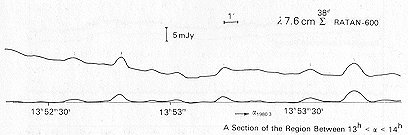
Figure 6.2 A small section of a scan at 7.6 cm (average
of 38 scans). It is also clearly evident here that the sky is "empty" between
the sources, and that the radiometer noise dominates, with a dispersion
of about 0.5 millijanskys. The upper curve is the initial data set, while
the bottom is after removal of the low-frequency background.
the region between the discrete sources do not differ strongly from those expected from Table V.I, if one overlooks the low-frequency fluctuations. We shall now discuss what procedures can be used to get closer to the "ideal" sensitivity, and make a quantitative estimate of what signal-to-noise ratio (S/N) can be obtained in practice. In this section, we are interested in small scales, so that the most troublesome interference – the anomalous low-frequency fluctuations – can be filtered out up to a rather high frequency – approximately 0.025 Hz (which corresponds to scales of ~ 10 l/D). Of course, high frequencies beyond the cutoff frequency of the antenna, must also be filtered out. The preparation of the initial set of data recorded at 7.6 cm with a time constant of 1.3 s ccnsisted of decreasing the interval between readings to 1.8 s and removing the noise spikes (Section 6.1). The filtering itself can be carried out by various methods; one of them, proposed by Heeschen, consists of the following operations:
– smoothing with the function (sin x/x) (suppressing frequencies above
fc).
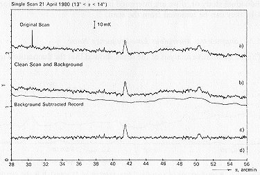
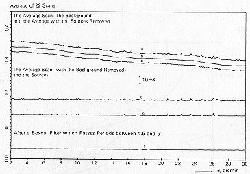
The basic operations which were carried out on the Experiment Cold
scans in an analogous data reduction method are shown in Figs. 6.3 and
6.4.
Another convenient method of identifying the sources and suppressing
the low-frequency fluctuations is the second-diAerence method. We shall
discuss this method in more detail – what kind of filter it corresponds
to, and what -ind of S/N ratio is obtained. The procedure of constructing
the second differences of the initial set of data
corresponds to convolving the initial set of data with delta functions distributed as shown in Fig. 6.5(a). The frequency response curve of such a filter is the Fourier transform of this pattern of delta functions
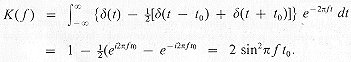 (6.1)
(6.1)The basic operations which were carried out on the Experiment Cold scans in an analogous data reduction method are shown in Figs. 6.3 and 6.4.
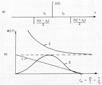
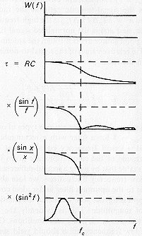
The following are shown in Fig. 6.5(b): (1) the spectrum of a signal
corresponding to the antenna frequency response; (2) the noise spectrum,
with a sharp increase at low frequencies; (3) the frequency response of
filter (Eq. (6.1)). The maximum of the frequency response curve obtained
in this way lies at a frequency 1/2 fc this is nearly the optimum
for the combination of noise and signal spectra under discussion. We remind
the reader that the signal spectrum at the output of the radiotelescope
and radiometer is the spectrum of the response of the antenna to the passage
of a point source. If the response is a function of the form (sin x/x),
which corresponds to the idealized case of a uniform electric field distribution
over the antenna aperture,* the signal spectrum J(F) is described by the
function (curve I in Fig. 6.5(6))
For a signal with this spectrum, the optimum output filter yielding
the maximum signal-to-noise ratio under ideal conditions (i.e., in the
absence of anomalous low-frequency fluctuations) would be one like (Eq.
(6.2)); see also Table VI.I. As we shall show below, using a filter with
a response curve which suppresses both low and high frequencies (Eq. (6.1))
allows one to come very close to the "ideal" sensitivity in problems involving
observations of sources with small angular diameters. However, such a filter
would be optimum if the useful signal possessed a spectrum of the same
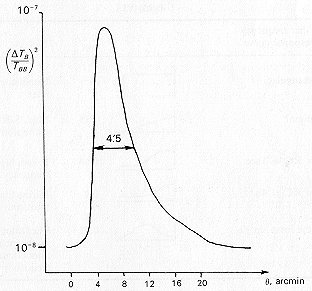
form, with a steep slope at low (near zero) and high frequencies. The expected
fluctuations in the temperature of the cosmic background
DTB/TBB have a spectrum of this type (in one
variant), with a maximum on scales of 5 – 10arcmin (Fig. 6.6). Moreover,
this range of scales is the least aA'ected by external interference (see
Fig. 5.1). This is why an attempt was made to search for fluctuations in
the cosmic background on these particular scales within the framework of
Experiment Cold.
Returning to the problem of identifying point sources, we shall now
find out whether we lose much in signal-to-noise (relative to observations
under ideal conditions, when the noise is thermal (i.e., in comparison with Table V.I) by using a filter of the form (6.1) under conditions in which there is an anomalous increase in the noise at low frequencies. In order to find this out, we use the equation for the signal-to-noise ratio at the output of a radiometer for a given (arbitrary) type of output bandpass and signal spectrum (Esepkina, Korol'kov, and Pariiskii, 1973 (Chapter II, Eq. 20)):
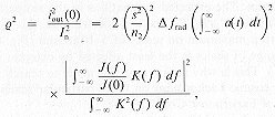 (6.3)
(6.3)where J is the signal spectrum, i.e., the Fourier transform of
the outputsignal current iout; K2( f) is the
shape of the output bandpass in terms of power;- s/n is the signal-to-noise
ratio at the radiometer output ![]() is the high-frequency bandwidth of the radiometer, and a(t) is the
normalized signal function (the flux of the signal as a point source drifts
through the antenna pattern). Since we are interested in relative values
of the signal-to-noise ratio
is the high-frequency bandwidth of the radiometer, and a(t) is the
normalized signal function (the flux of the signal as a point source drifts
through the antenna pattern). Since we are interested in relative values
of the signal-to-noise ratio ![]() , we shall write Eq. (6.3) in the form
, we shall write Eq. (6.3) in the form
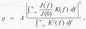 (6.4)
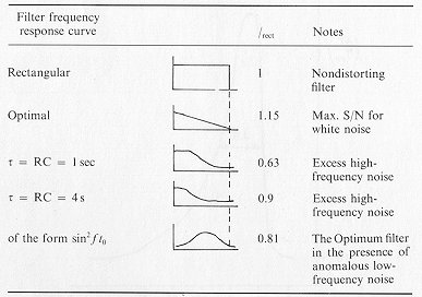
(6.4)and calculate relative values of ![]() for various types of output filters, and assuming that
for various types of output filters, and assuming that ![]() rect
= 1 for a filter with a rectangular frequency response curve and
a cutoff frequency equal to that of the antenna, fc = D/l.
The results of the calculations are given in Table VI.I. It follows from
this table that by using a second-difterence filter to remove the anomalous
low-frequency fluctuations, we lose about 30% in sensitivity compared
to the optimum filter under ideal conditions, but the gain due to suppressing
the low frequency fluctuations amounts to several orders of magnitude.
This is evidently the limit which the observer should strive to reach under
real conditions. Other methods of filtering out the low frequency noise
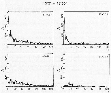
should yield similar results. To conclude this section, we show the procedure
of transforming the output noise spectrum at successive stages in the filtering
process in Fig. 6.7. The first stage in this process is performed in analog
form by an RC filter at the radiometer output, the next is the procedure
of compressing the readings (equivalent to multiplying the spectrum by
(sin f)/f), followed by convolution with a function of the form (sin x)/x,
which is equivalent to multiplication by a boxcar function in frequency
space, and, finally, filtering by the second-difference method. In Fig.
6.8, the output noise spectrum is shown at various stages in the filtering
performed by V. V. Vitkovskii on one section of an actual scan in
the course of reducing the materials from Experiment Cold.
rect
= 1 for a filter with a rectangular frequency response curve and
a cutoff frequency equal to that of the antenna, fc = D/l.
The results of the calculations are given in Table VI.I. It follows from
this table that by using a second-difterence filter to remove the anomalous
low-frequency fluctuations, we lose about 30% in sensitivity compared
to the optimum filter under ideal conditions, but the gain due to suppressing
the low frequency fluctuations amounts to several orders of magnitude.
This is evidently the limit which the observer should strive to reach under
real conditions. Other methods of filtering out the low frequency noise
should yield similar results. To conclude this section, we show the procedure
of transforming the output noise spectrum at successive stages in the filtering
process in Fig. 6.7. The first stage in this process is performed in analog
form by an RC filter at the radiometer output, the next is the procedure
of compressing the readings (equivalent to multiplying the spectrum by
(sin f)/f), followed by convolution with a function of the form (sin x)/x,
which is equivalent to multiplication by a boxcar function in frequency
space, and, finally, filtering by the second-difference method. In Fig.
6.8, the output noise spectrum is shown at various stages in the filtering
performed by V. V. Vitkovskii on one section of an actual scan in
the course of reducing the materials from Experiment Cold.
6.3. Conclusion
Removing the noise spikes and filtering out the low-frequency anomalous noise allow us to successfully identify point sources when the log N – log P curve is extremely flat, obtaining system sensitivities which come very close to the ideal sensitivity in the process. It is clear
that the observer should not expect an increase in the signal-to-noise
ratio above that of the standard optimal filtering methods for the ideal
case (i.e., thermal noise alone). Moreover, he should make sure that he
has not "over-filtered" his data.
A classical, well-studied example of a method for the optimal removal of thermal noise at the radiotelescope output (when searching for faint point sources) is convolution with the point source response. However, as we pointed out above, the whole problem is that the noise at the radiometer output has nothing in common with classical thermal noise, and, in the opinion of many experienced observers, the lion's share of
the difficulties in data reduction occur in "editing" (rather than reducing) the initial data set, i.e., in fact, in the process of making the noise approximately thermal and in correctly determining the "weights" of the harmonics in the spatial-frequency spectrum.
6.4. Protocluster Scales, i.e., on the Order of 10 Arcmin
These scales are important because they are similar to the scales of "protoclusters" of galaxies, the sizes of the background X-ray emission in nearby galaxy clusters, and the scales of the halos around strong radio sources. These scales diH'er from the smaller ones because of the necessity of filtering out the anomalous low-frequency fluctuations more carefully, and because of the absence of sufficiently reliable a priori information on the form of the signal function, as in the case of point sources (the antenna pattern). The major sources of interference on these scales are:
6.4.1. Preparation of the data set The preparatory operations included removing noise spikes and increasing the sampling rate (to roughly twice the characteristic sampling rate of the radio telescope), i.e., as in Section 6.1. An additional preparatory operation at this stage is the removal of radio sources. The point sources can be taken into account fairly confidently when they pass through the center of the beam (with dimensions of 1' x 10'). Identifying such sources was, in fact, the goal of the work described in the preceding section. We are now interested in the larger scales, and strong sources far away from the beam in declination, which pass through the edge of the antenna beam, make the situation more complicated. They correspond to features in the scans whose dimensions may reach tens of arcminutes. In order to identify and remove such sources, observations of the same band of sky were carried out using a sector of the RATAN shifted in azimuth by 30o. After determining the declination of the feature from the observations at the meridian (azimuth 0") and at an azimuth of 30o (as was done for the right ascension interval between 13h and 14h), it was possible to verify whether the observed apparent size of the feature agreed with the calculated size (the calculated antenna pattern is shown in Fig. 3.8). The majority of the features observed satisfy this theoretical relationship. Thus, it turned out to be possible to remove not only the sources identified by the method of Eq. (6.1), but a significant fraction of the distant interfering sources as well.
the entire low-frequency portion of the signal spectrum from 0 to –1/2
fc as well as the high frequencies above fc
is removed (integrating from –1/2 fc to fc).
We then obtain an identical result for the case of the optimal filter and
the filter with a rectangular frequency response:
i.e., because of the strong cut-off of the low-frequency portion, we lose almost a factor of three compared to the ideal case; however, in the process, we decrease the original dispersion on protocluster scales by several orders of magnitude. We believe that this method of "normalizing" over boxes comparable to the characteristic "intrinsic time interval" of the object under study is similar to the well-known "rank criteria" for dealing with interference, and has an adequate logical basis.
When using sufficiently powerful computers, a two-dimensional statistical
analysis can be carried out. Extremely deep studies, as a rule, are carried
out via many repeated observations of the same region of sky. It is always
possible to represent the results of such observations in the form of a
rectangular matrix of numbers, where each row contains readings spacing
by the "intrinsic time interval" of the antenna and each column gives the
values of the antenna temperature for the same region of sky, but at difterent
times. Thus, a matrix with dimensions m x n (where m is
the number of independent readings in a realization, and n is the
number of realizations) is constructed. For the clusters, we performed
a statistical analysis (removing the normal noise) along the rows. After
removing the low-frequency noise on all the scans, it is possible to carry
out an analogous procedure along the columns as well – all of the deviations
from the mean reading must follow a normal distribution. The departures
should be ascribed to interference, and the corresponding readings on the
appropriate scans should be replaced by the average value of the column.
For white noise, the parameters of the normal law should be identical for
the rows and columns. Therefore, observers in the US use this circumstance
to apply the Fisher criterion when searching for Gaussian noise from the
3-degree background.
6.5. Large Scales – The Background Emission of the Galaxy
The main problems here were the large-scale fluctuations in the cosmic background radiation and the background emission of the Galaxy. The chief source of interference is the unstable emission from the atmosphere. On very large scales, the emission of the Galaxy itself becomes perceptible. The first and second harmonics of the brightness distribution in the band 0h < a < 24h are due to the emission of the Milky Way, and they dominate the spatial frequency spectrum of the Galaxy, while the tropospheric structure function becomes saturated on scales of – 15o (for an average wind velocity ~ 7 km s-1).
On these same scales, numerous instrumental drifts due to variations in the ambient temperature and the temperature in the input circuits, as well as the stability of the amplifiers, were present. Much effort was expended, and the ingenuity of those who developed the radiometer was manifested in the struggle for the internal stability of the radiometer (Berlin and Gol'nev, 1982). Then, a correlation between the hourly fluctuations and the temperature inside the receiver cabin was noticed. It was later noticed that these fluctuations were significantly higher at the output of the 8.2-cm radiometer, for which the losses at the input are higher. This allowed these fluctuations to be interpreted as variations in the emission from the feed horns themselves. The unacceptable ripple at the radiometer output, with a period of 1.3 s (the refrigerator cycle), and the instability in the temperature within the parametric amplifier cryostat (which led to drifts with an amplitude of up to 100mK) were removed. An attempt to take the atmospheric conditions into account using sensors for the outside temperature, pressure, and humidity (which were recorded every hour by the observers on duty during the entire deep survey cycle) turned out to be unsuccessful (perhaps the observations were not accurate enough). Nevertheless, we were able to show that the dominant drifts on time scales of 1h are not connected with these parameters. We note that the eftorts of the engineers in their work on the receiver were clearly successful; fluctuations of unknown nature, with a characteristic time scale of order 1 h and a rather low amplitude (<=100mK) are what we are discussing here. An example of a night-time scan many hours long made in good weather (Fig. 3.2) bears rather eloquent testimony to this fact, since it is clear that these are features of "celestial" origin.
One of the strongest sources of interference on large scales is the effect of the direct incidence of solar radio emission on the primary feed of the radio telescope. The contribution from this effect may reach 100 mk at unfavorable times and leads to rapid changes in the signal level at sunrise and sunset, as well as when the sun goes behind and comes out from behind the secondary mirror of the radio telescope. Evidently, this effect can be decreased by using a primary feed with less scattering, and by adding simple screens to the edges of the secondary mirror which are matched to the field distribution in this region (see the results of the work of Maiorova, Korol'kov, and Stotskii in Section 3.4). In Experiment Cold, it was also necessary to stop observing for about two hours as the sun passed through the meridian. This region of the sky was illuminated by the sun through the sidelobes of the antenna pattern (see Ignat'eva et al., 1982). Some of the eftects may be due to surface errors and the cracks between the elements; in Experiment Cold, the cracks were screened to reduce the antenna noise temperature, but the screens introduced phase errors and therefore also increased the scattering near the main beam of the antenna pattern. In Experiment Cold, only 175 elements of the north sector were used, rather than the entire sector (225 elements); the secondary mirror was
designed to illuminate 225 elements. This led to a sharp decrease in
the field distribution over the aperture, which also increased the amount
of scattering near the main beam of the antenna.
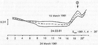
Despite all of the difhculties listed above, we attempted to construct a complete 24-h profile of the antenna temperature distribution along our band on the sky. We "sewed together" the points within 1 h before and 1 h after the culmination of the Sun, as well as the 2 – 3 min gaps for calibration and compensation at the end of each hour of observations. The two quietest records in the entire set (19 and 24 March, 1980), which turned out to be similar (except for the strong features which vary with solar time and are almost a fortiori connected with the disappearance of the feed into the "shadow" of the secondary mirror), were selected. These 24-h-long scans are shown in Fig. 6.10. The repeatability of the curves is encouraging. The next stage consisted of carefully classifying all of the scans according to quality; the average curve resulting from selecting the 13 best 24-hour-long curves was used to analyze the large-scale distribution of the background emission of the Galaxy (Fig. 8.2). The Galactic component of the background will be discussed in more detail in Section 8, but we shall note here that on individual 24-h-long scans under good atmospheric conditions, the Galactic emission dominates on scales of 30o – 360oC. We also note that in Experiment Cold, a complete cross-section through the Galaxy at centimeter wavelengths was obtained for the first time. Our experience in identifying the Galactic background showed that by using methods for removing the atmospheric emission, one can hope to make the accuracy of ground-based background observations close to that of space-based studies (at least at centimeter wavelengths), and actually obtain the sensitivity of the new-generation radiometers in practice. Moreover, this suggests that it is necessary to use shorter wavelengths to study the extragalactic background radiation on larger scales.
6.6. Scales Comparable with the Size of the Horizon at the
Recombination Epoch (0.5 – 2o)
These scales are of particular interest in connection with the fundamental question of the causal relationship between sections of the Universe on scales larger than the size of the horizon at the recombination epoch, and touch on key problems of singularities, as well as modern "Grand Unification Theories" (see, for example Novikov, 1983). Diffuse Galactic objects (H II regions and SNR's), superclusters, and the "voids" in the Universe also occur on these same scales. On these scales, we intended to use a procedure for removing atmospheric
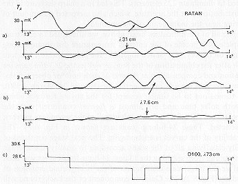
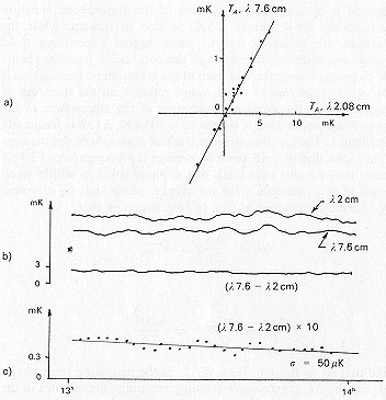
However, it unexpectedly turned out that the dominant noise energy on these scales at 7.6 cm was due to real features on the sky, repeatable from one observation to another; these features were also visible at 31cm (see Fig. 6.11). The correlation between these wavelengths becomes even more obvious if the discrete sources and the very-low-frequency noise (on scales larger than 5o) are removed (see Fig. 6.12(a)). We therefore initially decided to remove the noise which was correlated at wavelengths of 31 and 7.6 cm from the scans (Fig.6.12(b)). It was
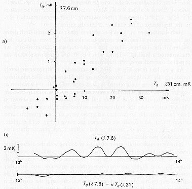
Figure 6.12 The effectiveness of the removal of Galactic noise from the 7.6-cm data. (a) Establishing the correlation between the fluctuations at 31 cm (average of 65 days) and 7.6 cm (average of 22 days). The correlation coefficient is greater than 0.8. (b) The result of subtracting the 3 l-cm data from the 7.6-cm data using the slope determined from the regression curve in (a). Noise remains on scales of 0.o8- 5o.
possible to select an amplitude for the filtered scan at 31 cm such that simply subtracting it from a scan of the same section of sky at 7.6 cm led to almost a factor of ten decrease in the dispersion at 7.6cm on scales of 1o – 2o. It was immediately observed that after taking the experimental correction for the spillover loss at 31 and 7.6cm into account, the procedure for choosing the amplitude is identical to the assumption that the emission from the features visible in Fig. 6.11 is synchrotron in nature, with a brightness temperature spectral index of 2.55, which is very similar to the spectral index of the Galactic background emission at latitudes greater than 10o(see Section 8). We attribute these features to structure in the Galactic background emission. Their characteristic size is approximately 1o – 2o, and their amplitude at 7.6cm is about 1 mK. Their relative amplitude in the section 13h < a < 14h (latitude of approximately 60o) is approximately 1 – 2% of the brightness of the Galaxy in this direction.
Such fluctuations in the sky brightness place substantial limitations on the sensitivity of radiotelescopes to scales of 1o– 2o even in the coldest region of the Galaxy. Thus, for single-frequency observations, we encountered a limit of ~ 1 mK, which is 50 – 100 times worse than the expected thermal noise for Experiment Cold.
As is evident from Fig. 6.12(b), we succeeded in almost completely removing
this "Galactic" noise by using the 31-cm data. The remaining emission at
7.6 cm is correlated (as was expected) with the emission at shorter wavelengths.
The regression curve for the relationship between the remaining emission
at 7.6 cm and the emission at 2cm is shown in Fig. 6.13(a). Noting the
high correlation coefficient, we subtracted the 2-cm data from the 7.6-cm
data using the slope of the regression curve (Fig. 6.13(b)). As a result,
we obtained the curve in Fig. 6.13(c). Here, s ![]() 50 mK, i.e., the dispersion is only a few times
greater than that expected in the ideal case (Table V.I).
50 mK, i.e., the dispersion is only a few times
greater than that expected in the ideal case (Table V.I).
In order to successfully make progress in dealing with the atmospheric noise, the Galactic noise, and the noise from the ground, it is necessary to have several extremely sensitive radiometers observing simultaneously, and highly accurate temperature, pressure, and humidity sensors. Taking all of these sources of noise into account can only be carried out by the method of least squares, choosing the correlation coefficients with the other wavelengths in such a way that the mean square deviation at the wavelength being studied is a minimum. Naturally, this should be done after removing the uncorrelated interference and the discrete sources.
In order to attract experts to this important problem, we remind the
reader that in solving this problem rather efficiently, we simultaneously
solve the no less fundamental problem of the phase correction of images
in interferometer networks. Since ![]() ,
and
,
and
6.7. Conclusions
We shall now summarize the analysis of a data set averaged over 22 days of observations under good and fair conditions.
When studying point sources at 7.6 cm at intermediate elevations in the standard mode, it should be kept in mind that about 20% of the sky is filled with radio sources with flux density greater than 1 – 2mJy. Regions where the thermal radiometer noise dominates up to fractions of a mJy are frequently visible between the sources.
Finally, there are drifts on scales of 1 h, which were not successfully identified and whose amplitude is at least ~10mK (sometimes reaching 100mK) under good atmospheric conditions.
In order to come as close as possible to the noise of an "ideal" radiometer (more precisely, the "ideal" noise of a real radiometer at 7.6 cm) the RATAN-600 should be equipped with several new-genera-tion radiometers. Then, in a multi-frequency observing mode, it is possible to develop the mathematical method needed to realize the potential of the RATAN-600. Partial success can already be achieved using such a mathematical method with the present set of radiometers.
Finally, we saw that it is dangerous for the observer to try to dodge the problems in the struggle to approach the sensitivity in Table V.I. The general methodological lesson of Experiment Cold is that the noise from all of the sources of interference should be studied and methods for removing them should be evaluated first, and then it should be decided whether it is realistic to propose a certain experiment. From the experience of Experiment Cold, we believe that a search for the optimum radio-astronomical wavelength region for solving a particular problem should include a discussion of the methods of dealing with the sources of interference (dealing with Ssi , rather than the components of Tsys).