|
|
|
|
|
The main goal of Experiment Cold was to make an attempt to significantly increase the accuracy with which the degree of isotropy in the sky brightness at centimeter wavelengths is measured. The dominant contribution to the average sky brightness at 7.6 cm comes from the iso-tropic component of the cosmic background blackbody radiation, even at low galactic latitudes. This radiation has a brightness temperature of approximately 3 K and dominates over all other forms of radiation in energy density (and even more so in terms of number of photons per unit volume). In "orthodox" cosmology, this radiation is due to the emission from the hot plasma in the first million years of the existence of the Universe after its "creation" in the "Big Bang" theory. The chief (and most attractive) result of this interpretation of the 3-degree background is that it gives us a unique opportunity to construct a picture of the Universe in those remote times after constructing a detailed radio image of this background. In essence, this is an attempt to construct an analog of the Palomar Sky Survey (which reflects the structure of the Universe "today", i.e., in the vicinity of our Galaxy), but for an epoch corresponding to red shifts of about 1000, when the age of the Universe was only several hundred thousand years. In those remote times (according to the standard models), the Universe was filled with an almost homogeneous plasma, and small inhomogeneities in the density, temperature, velocity field, and gravitational potential in this medium subsequently led to the formation of all of the presently observable structure in the Universe (galaxies, clusters, etc.). The first studies of the possibility of detecting protogalaxies were carried out by Silk (1967). In the same year, Conklin and Bracewell (1967) showed that the background was uniform to within 3.6 mK. Between 1967 and 1980, we carried out a series of observations of the small-scale fluctuations in the 3-degree background with the prototype for the RATAN-600 (the Large Pulkovo Radio Telescope), using a significantly more sensitive radiometer than was available to Bracewell and Conklin (see Pariiskii et al., 1968, 1970, 1972, 1973, 1977, 1978, 1981, and Berlin et al., 1982). Our first limit was smaller than 1 mK.
It soon became clear that the nature of the small-scale anisotropy of the 3-degree background might be related not just to the structure of the Universe at z = 1000, but also to many fundamental questions about the singularity, theories concerning the Grand Unification of all forms of interaction, the theory of the formation of radiation and matter (and even humanity) in the Universe, the processes which occurred after the recombination of hydrogen, the search for large-scale gravitational waves, determining the rest mass of the neutrino, etc. Therefore, many radio observatories are continuing their efforts in the search for aniso-tropy in the 3-degree background, and, large space experiments are even being planned in the USSR and abroad (see the complete review by Melchiorri (1982)).
Tens of experiments on the small-scale anisotropy of the 3-degree background have been carried out since 1967, and, as a rule, an upper limit has been set on the amount of inhomogeneity in the background. There are only three reports of positive results: from the NRAO (U.S.) on protogalaxy scales (Martin and Partridge, 1980), from the Max Planck Institut fuer Radioastronomie (FRG) on protocluster scales (Wielebinski, 1982) and from Melchiorri's group in Italy (Florence) on scales comparable to the "horizon" at the recombination epoch in an empty Universe (a scale of several degrees (Zel'dovich and Syunyaev, 1970)). At this point, we remind the reader that on very large scales, the dipole component in the distribution of the 3-degree background is believed to be quite well-established, while the data on the quadrupole component is contradictory: at IAU Symposium 104 (Crete, Sept. 1982), Wilkinson showed that the latter can be completely explained by Galactic emission. At the same meeting, Melchiorri claimed that a large "spot" in the 3-degree background had been observed toward the Virgo supercluster.
In Experiment Cold, the main emphasis was placed on searching for "protoclusters"
– i.e., searching for temperature variations on scales of 5' – 10'; however,
at the same time, we were able to determine the amplitude of the fluctuations
on both larger and smaller scales. In Experiment Cold, we decreased the
upper limit on the small-scale anisotropy by a factor of 100 relative to
the first attempts in the U.S. (Pariiskii and Pyatunina (1970), DTB<=
0.7x10⁻³ K), lowering the limit to DTB<=3x10⁻⁵
K. We shall now describe how this was accomplished.
9.2. Obtaining the Raw Data
As we mentioned above, our main goal when choosing the observing method was to obtain the highest possible radio telescope sensitivity to the surface brightness of regions of the sky comparable to the scale of protoclusters, i.e., 4' – 10'. The major factors which interfered with this goal were discrete radio sources, atmospheric emission, interference, and the like. As we say, the behavior of the "number of sources – flux density" curve at centimeter wavelengths between 1 and 10 mJy allowed us to correct for the influence of background radio sources by simply subtracting them from the entire set of raw data. An example of the procedure by which the radio sources were subtracted was shown in Fig. 6.4. At the ultimate sensitivity of the radio telescope, about 10 – 20% of the sky is occupied by sources of radio emission at 7.6 cm. The structure of the 3-degree background must be studied in the "gaps" between the radio sources.
As we discussed in Section 6, the background emission "between" the
radio sources at 7.6 cm turned out to be correlated with the background
at 31 cm. This correlation is particularly clear on scales of 1o
– 2o (see Fig. 6.1). Since the spectrum of the correlated components
of the variations in the background emission is almost the same as that
of the Galactic background emission (see Fig. 8.3), we attributed these
varia-
|
|
|
|
|
|
h1, is a factor which takes into account the transformation from ntenna temperature to brightness temperature for extended objects;Thus, the estimate
h2 is a factor which takes into account the ratio between the size of the inhomogeneities (7') and that of the antenna pattern of the radio telescope in the vertical direction. As we showed in Section 4.6, coefficient h10.75, and the factor h2 is roughly 0.25;
N is the number of independent readings in the data set. In our example, N = 64. The factor ofin the denominator takes the fact that the distribution of inhomogeneities in the beam is random into account; and,
UD is the quantile of the distribution, assumed to be 2 in this case.
It is clear that when the inhomogeneities being searched for in the background are much larger than the radio telescope beam,
For inhomogeneities in the background whose size in the vertical direction is smaller than the antenna beam, an additional factor h2, must be introduced (Section 4.6):
(a) the "thermodynamic" loss for a single inhomogeneity with respect to h2 because radiation is received from a region Fiy and reemitted by the antenna over the region FAy andAs a result we lose a factor of(b) a statistical gain of a factor of
, since there are FAy/Fiy inhomogeneities within the beam at the same time.
Table IX.II was complied using the critical density of the universe and the relation
|
|
|
|
|
|
|
|
|
|
on the scale of protogalaxies; this is a factor of 10 lower than the value obtained at 1 1 cm for these same scales in the U.S. Thus, direct observations on small scales are also inconsistent with the NRAO Observations (Martin et al., 1980). This result at 1.38 cm is a factor of 20 Worse than the extrapolated 7.6 cm data, but is independent (more precisely, almost independent) of the statistical properties of the inhomogeneities in the background radiation on scales larger than 7".
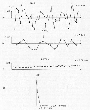
Figure 9.1 A comparison of the 1980 RATAN-600 results
in studying the isotropy of the three-degree background with Partridge's
(1980) best data: Curve (a): The average of 118 drift curves of a small
region of the sky with readings averaged over boxes 20 s long in right
ascension. Curve (b): the same data, smoothed, with the sampling rate reduced
by a factor of four. Additional careful data reduction allowed Partridge
to set limits of 2 x 10⁻⁴ and 6 x 10⁻⁵ on DTB/TB
for scales of ~4' and 7', respectively. The lower curve is a portion of
the data from Experiment Cold at 7.6 cm, with scales smaller than 4'.5
and larger than 9' suppressed from our data; we estimate our limit to be
10-5 to the same level of significance – 2s.
9.3. Comparison with Other Observations
Our observations are not inconsistent with earlier published data on
upper limits to the fluctuations in the background radiation. We obtained
an improvement of a factor of 5 – 8 over our previous observations at the
RATAN-600 (Pariiskii et al., 1977), and a factor of 6 – 10 over Partridge's
recent results. Figure 9.1 shows a comparison of Partridge's initial data
sets and the results of Experiment Cold. The upper curve is taken from
Fig. 2 of Partridge (1980), the middle curve is where we have decreased
the sampling rate in Partridge's data set by a factor of 4, and the upper
curve is a portion of the data (5% of the data set) from Experiment Cold.
It is curious that the integration times for the emission from a single
inhomogeneity on a scale of 4', as well as the data filtering windows are
similar for Partridge and us in this sample, since Partridge's double-beam
scanning yields a filter window from 3'.6 to 9', while our filtering on
the computer was carried out with a window 4'.5 to 9'. However, our brightness
temperature dispersion is 10 times lower than for Partridge. This is not
so much a merit of the antenna as the radiometer we used in Experiment
Cold. We remind the reader that Partridge (1980) had Tsys =
570K and Df = 1 GHz. We have Tsys
= 37K and Df = 500MHz.
We have already mentioned that three reports of detections of fluctuations
in the 3-degree background have been published. Let us list them:
(a) Martin, Partridge and Rood (1980). Fluctuations at 11 cm were observed at the NRAO on scales of 13":
(b) Melchiorri (1982) has observed variations in the background on scales of several degrees at a level of
in the wavelength range 0.5 – 2mm.(c) The observers at Effelsberg have reported (Wielebinskii, 1982) observing fluctuations at a level of
– the NRAO result can be explained by the difficulty of taking confusion noise into account because of influence of the faint, but broad scattering in aperture – synthesis systems;A few words about corrections for instrumental effects. First, a lack of coordination between the actions of observers and theoreticians is evident. Theoreticians try to make their calculations approximate observations, and include the effects of smoothing by hypothetical antenna beams. Observers, who have in hand information about the actual instrumental effects, correct their observations and compare them to the original theoretical studies. Sometimes, this leads to confusion – the smoothed theoretical fluctuations are compared with the corrected observed fluctuations, etc. Secondly, observations of other people should be corrected with extreme care – this leads to distortion of the facts. Thus, the good intentions of Partridge (1980) to create a uniform table of observational data went wrong for at least three reasons:
-Melchiorri's result can be explained by emission from dust in the region between 0.5 and 2mm, which is not ruled out by the author himself;
– the result obtained in Bonn has as yet only been briefly reported at the working group "RATAN-600-D100" (Leningrad, 1982), but it seems to us that the "mixed" statistics of the noise at 2.8 cm (radiometer white noise and the increasing structure function of the atmospheric emission) may explain the Effelsberg result.
(a) Partridge possessed erroneous information about what telescope the observations were carried out on; the radio telescopes at Pulkovo, the NRAO and JPL were confused;Table IX.III Summary table of fluctuations in the Microwave Cosmic Background Radiation
(b) the number of independent scans of the same piece of sky was confused with the number of independent pieces of data in the data set; and,
(c) the concepts of the effective area of a radio telescope and aperture efficiency were confused. This strongly distorted the relationship between antenna temperature and brightness temperature (even in Partridge's measurements).
|
|
l2 cm |
|
|
|
| 1 | 2 | 3 | 4 | 5 |
| 1
2 3 4 5 6 6a 7 8 9 10 11 l2 13 14 15 16 17 18 19 20 2l 21a 22 22a 23 24 24a 25 26 27 28 29 30 31 32 33 |
Berlin et al., 1983
Berlin et al., 1983 Martin et al., 1980 Berlin et al., 1983 Partridge et al., 1983 Martin et al., 1980 Goldstein et al., 1976, 1979 Kellermann et al., 1983 Berlin et al., 1983 Kellermann et al., 1983 Berlin et al., 1983 Penzias et al., 1969 Boynton et al., 1973 Pigg (see Boynton, 1981) Pariiskii and Pyatunina,1968 Rudnick, 1978 Carpenter et al., 1973 Epstein, 1967 Pariiskii, 1973 Partridge, 1979 (see Smoot, 1980) Lake and Partridge, 1980 Wilkinson, 1983 Uson and Wilkinson, 1984 Birkinshaw, 1981 Uson and Wilkinson, 1984 Berlin et al., 1983 Pariiskii et al., 1977 Wielebinski, 1981 Partridge, 1983 Ledden et al., 1980 Stankevich, 1974 Conclin and Bracewell,1967 Seielstad et al., 1981 Epstein, 1967 Pariiskii et al., 1977 Lasenby and Davies, 1983 Pariiskii et al., 1977 |
7.6
1.38 3.7 7.6 6 11 2l 6 7.6 6 7.6 0.35 0.35 2 3.95 2 3.56 0.34 2.8 0.97 0.97 1.5 1.5 2.8 2 7.6 3.95 2.6 0.97 6.3 11 2.8 2.8 0.34 3.95 6 3.95 |
7''-20'' 4'' 4''-6'' 6'' 13'' 17" 18" 18" 1' 1' 1'.3 1'.5 1.'25 I'.4 2' - 20' 2.'3 - 1o 3' - 1 2.'5 3'- 1' 3.'6 3.'6 4.'5 4.'5 4.'5 4.'5 4'.5 - 9' 5' 7' 7' 7' 8' - 19' 10' 11' 12'.5 12'.5 10' 20' |
< 3 x 10⁻¹*
< 10-3 < 4 x 10⁻³ < 2 x 10⁻⁴ < 10-3 7 x 10⁻² < 3 x 10⁻³ < 7.8 x 10⁻⁴ < 7.8 x 10⁻⁵* < 2.1 x 10⁻⁴ < 2.2 x 10⁻⁵ < 4.0 x 10⁻⁴ < 1.8 x 10⁻³ 7.5 x 10⁻⁴ 2.3 x 10⁻⁴ 2.3 x 10⁻⁴ 7.0 x 10⁻⁴ < 5.0 x 10⁻³ < 5.0 x 10⁻⁵ < 2.0 x 10⁻⁴ < 10-4 < 1.1 x 10⁻⁴ < 4.5 x 10⁻⁵ < 2.5 x 10⁻⁴ < 3 x 10⁻⁵ < 10-5 < 8.0 x 10⁻⁵ 4.0 x 10⁻⁵ < 6.0 x 10⁻⁵ < 6.0 x 10⁻⁴ < 1.4 x 10⁻⁴ < 1.8 x 10⁻³ < 2.5 x 10⁻⁴ < 1.0 x 10⁻² < 4.0 x 10⁻⁵ < 3.0 x 10⁻⁴ < 3.0 x 10⁻⁵ |
| 34
35 36 37 38 39 40 41 42 43 44 45 46 47 48 49 50 50a 50b 51 52 53 54 55 56 57 58 59 60 61 61a 62 |
Lasenby and Davies, 1983
Lasenby and Davies, 1983 Carderni et al., 1977 Penzias and Wilson, 1965 Wilson and Penzias, 1967 Pariiskii et al., 1977 Lasenby and Davies, 1983 Conclin and Bracewell, 1967 Berlin et al., 1983 Berlin et al., 1983 Penzias et al., 1969 Pariiskii et al., 1977 Fabbri et al., 1980 Conklin and Bracewell, 1967 Conklin and Bracewell, 1967 Fabbri, 1980 (see Smoot, 1980) Smoot, 1980 Fabbri et al., 1982 Boynton et al., 1983 Smoot, 1980 Wilkinson, 1983 Partridge and Wilkinson, 1967 Dismukes, 1968 (see Partridge, 1978) Wilkinson et al., 1968 (see Partridge, 1978) Conclin, 1972 Boughn et al., 1971 Beery, 1968 (see Partridge, 1978) Wilkinson, 1983 Wilkinson, 1983 Berlin et al., 1983 Strukov and Skulachev,1984 Smoot, 1980 |
6
6 0.13 7.35 7.35 3.95 6 2.8 31 7.6 0.35 3.95 0.1 2.8 2.8 0.05 - 0.3 0.91 0.05 - 0.3 0.1 0.91 0.3; 1.2 3.2 3.2 3.2 3.8 0.86 3.2 0.13 0.65 - 1.58 7.6 0.8 0.91 |
30'
30' 30' 40' 40'-60' 50' 60' 1o 1o.5 1o - 5o 1o.5 2o.5 2o 2o 6o 6o 7o - 20o 40o ~ 40o 90o 90o 90o 90o 90o 90o 90o 90o 90o 90o 90o 90o 180o |
< 4.6 x 10⁻⁴
9.0 x 10⁻⁵ < 1.3 x 10⁻⁴ < 0.1 < 3.5 x 10⁻² < 2.5 x 10⁻⁵ < 2.3 x 10⁻³ < 2.0 x 10⁻⁴ 3.0 x 10⁻³ < 1.5 x 10⁻⁵ < 6.0 x 10⁻³ < 1.5 x 10⁻⁵ < 3.0 x 10⁻⁴ < 5.0 x 10⁻⁴ 1.2 x 10⁻³ 3.0 x 10⁻⁵ < 3.0 x 10⁻³ 3.0 x 10⁻⁴ ~ 3.0 x 10⁻⁴ < 5.0 x (10+-7) x 10-3 (10+-7) x 10-3 (0.7 +- 0.7) x 10-3 (1.48 +- 0.89) x 10-3 (0.5 +- 0.3) x 10-3 (2.04 +- 2) x 10-3 (0.7 +- 0.44) x 10-3 (0.2 +- 0.05) x 10-3 (0.2 +- 0.05) x 10-3 <10-3 < 7 x 10⁻⁵ (1.13 +- 0.13) x 10-3 |
| 63
64 65 66 67 68 69 70 71 72 73 |
Melchiorri and Melchiorri,1982
Berlin et al., 1983 Partridge and Wilkinson, 1967 Dismukes, 1968 (see Partridge, 1978) Wilkinson, 1968 (see Partridge, 1978) Conclin, 1972 Boughn et al., 1971 Henry, 1971 Beery, 1968 (see Partridge, 1978) Fabbri et al., (see Melchiorri, 1982) Cheng et al., 1979 |
0.91
7.6 3.2 3.2 3.2 3.8 0.86 2.9 3.2 0.13 0.9 - 1.5 |
180o
180o 180o 180o 180o 180o 180o 180o 180o 180o 180o |
|
In conclusion to this section, we list all published limits on the
3 K emission on all scales. The numbers in Table IX.III are given in the
order of increasing of the scale of inhomogeneity. The same numbers may
be found in Fig. 9.2. Here open circles correspond to the positive results,
filled circles to the upper limits. The dashed line connects all measured
and extrapolated RATAN-600 points. Extrapolation was done using the Conklin
and Bracewell method (1967). At the bottom of the figure the expected thermal
noise limit is marked for planning a new experiment with RATAN-600 and
1-year integration time.
9.4. Comparison with Theory
In this section, we will briefly compare our observations with the theoretical studies of the expected fluctuations in the 3-degree background which have been carried out over the last 15 years in the USSR and abroad. The authors are not cosmologists; our analysis of the situation at present is undoubtedly subjective, and only involves whether our observations are consistent or inconsistent with particular theoreti-
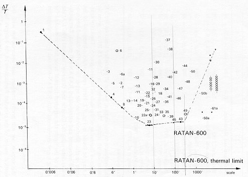
Figure 9.2 Observed limits on fluctuations in the microwave cosmic brackground radiation.
(1) How was the entire structured world around us (with galaxies, clusters, stars, and us) formed from the nearly homogeneous mass of light and matter at the recombination epoch?, andAt the beginning, it seemed to us that it would be possible to accurately determine when the galaxies were formed (Silk, 1967). In the linear theory, perturbations in the density(2) How could regions of the Universe further apart from one another than ct, where t is the age of the Universe, have the same temperature to better than 10-4 – 10-5 ? Such regions are not causally connected.
More rapid processes are necessary, and it is essential to take the non-linear stage into account. Ya. B. Zel'dovich's group showed the possibility and inevitability of the development of non-linear phenomena in an expanding Universe – the theory of the formation of "pancakes" and their fragmentation (Zel'dovich and Novikov, 1975). Of course, from the very beginning, the "vortex" theory actively used the non-linear stage in the transition from sound waves in a plasma filled with radiation (in such a plasma, the sound speed is close to the speed of light) to supersonic motions in the neutral gas after recombination (Ozernoi, 1967). Both the classical "pancake" theory and (even more so) Ozernoi's "vortex" theory led to unacceptably large fluctuations in the 3-degree background on protocluster scales. It seemed as if the finite mass of the neutrino solved the problem neutrino "proto-pancakes" form before the recombination epoch, and matter rapidly begins to fall into these potential wells immediately after becoming decoupled from the radiation. But, recent estimates (Zabotin, 1982; Nasel'skii et al., 1982) yield a fluctuation amplitude
The "steady-state Universe", with galaxies and clusters which have "always been in existence," has no such problems. However, the evolutionary model of the Universe seems so attractive from a theoretical point of view and so observationally well-founded, that one should, of course, continue to find ways of explaining the small fluctuations within the framework of evolutionary models. Rees and Hogan have suggested that the 3-degree background is not emission from the recombination epoch, but the result of the scattering of emission from already-formed objects against a gas-dust medium between us and these objects. This "reverses" the positions of the discrete objects and the region where the 3-degree background is formed. Hogan (1980) has carried out detailed calculations of the expected fluctuations in the background and predicts DTB/TB>(3–10)x10-5, and the fluctuations should depend on frequency. This value is also unacceptable (see Table IX.II).
Another alternative frequently discussed in the literature is to reject the fragmentation theories in favor of clustering theories. In this case (Zel'dovich, 1983), the eH'ects are smoothed out so strongly that the observational sensitivity must be increased a factor of 10 above that attained in Experiment Cold (to 10-6 in DTB/TB; see Boynton (1981), for example). Ya. B. Zel'dovich has recently proposed an effective way of combining all the potential of the Grand Unification theories with the observational limitations on the fluctuations in the background. In this scheme, massive neutrinos are replaced with more massive particles, which have a rest mass of approximately 1 keV (instead of 30 eV for the neutrino). These particles may be able to form large gravitational inhomogeneities on the scales of star clusters; these are then the primordial objects. These objects subsequently "cluster" in various ways into all of the successive levels in the hierarchy of objects in the Universe. Grand Unification theories predict the formation of such particles. We remind the reader that this theory also solves the problem of isotropy on large scales (larger than the scale of the horizon at the recombination epoch). There is now no "beginning", and the problem of "lack of time", which we mentioned earlier, does not exist; the Universe existed forever, expanding from a "strained vacuum" with a scale factor
9.5. A Search for Polarization in the 3-Begree Background
Immediately after Rees' (1968) theoretical paper appeared, we made an attempt (in the same year, 1968; Pariiskii and Pyatunina, 1971) to observe the predicted efTect – polarization of the 3-degree background due to multiple scattering both during the recombination era, and the "secondary heating" zone (Pyatunina, 1971) – using the Large Pulkovo Radio Telescope. Later experiments were described by Lubin et al., in 1979. These estimates were similar to the results of N. S. Soboleva (see Pyatunina (1971)) and led to a result of 0.8 mK on scales of a few degrees.
An accuracy of 0.3 mK on scales of 22' (which corresponds to the size of the "cells" in the cellular structure observed in the three-dimensional distribution of galaxies (see Einasto (1981), for example) was achieved in the Experiment Cold program at 3.9cm. This places firm limits on variations in the Hubble expansion at the recombination epoch, and during the secondary heating phase. The absence of polarization on small scales also places a limit on the energy density of low-frequency gravitational waves (see Dautcourt (1969); Doroshkevich, et al. (1977), and Basko and Polnarev (1980)). We remind the reader that the optical depth of the Universe is a factor of three smaller in polarized radiation than in unpolarized (Basko and Polnarev, 1980), so that we can see earlier stages in the evolution of the Universe. An analysis of our results shows that the measurements of the intensity fluctuations using the more sensitive 7.6-cm radiometer yield an even more precise upper limit to the polarization of the 3-degree background on small scales. Since only one plane of polarization was recorded,
Interpreting the polarization observations in the standard way to estimate the deviations in the motions from the Hubble expansion (Rees, 1968), we obtain an upper limit of ~10-6 on DH/H (H is the Hubble constant).